Why the Sediments Are There-Part 2: A Flood Regression Model

by Michael J. Oard, John K. Reed, and Peter Klevberg

 

Key Words: sediments,

continental margin sedimentation,

Late Flood Recession Model

 

Introduction

Reed et al. (2022) used isopach maps to show marine sediment distribution, to estimate total volumes, and to determine mean thicknesses (Table I and Figure 1). Current total marine sediment volume is mapped as 337,000,000 km ³ (Straume et al., 2019), providing a mean thickness of 927 m for the total ocean and ranging from 3044 m on the continental margins to 404 m for the deep oceans. We follow Straume et al. (2019) in defining (for the purposes of this paper) marine sediments as those starting at the present shoreline. However, estimates of the continental volume and average thickness often overlap some continental margin sediments. Moreover, some continental thickness estimates include Precambrian sediments, some Precambrian sediments, or none at all. Thus, estimates of the volume and average thickness of sedimentary rocks on the continents vary considerably between researchers and, as a result, we cannot use previous estimates.

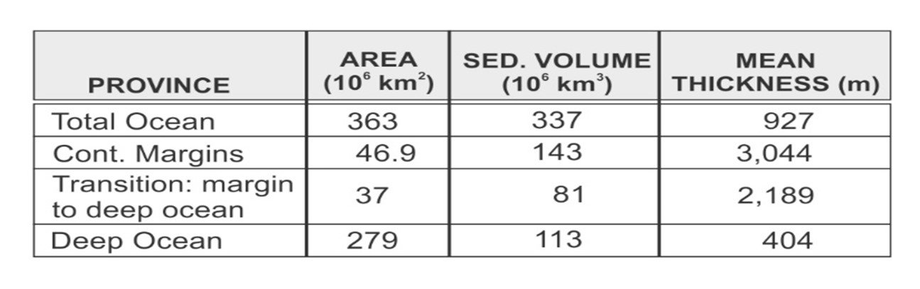
Table I. The three divisions of the ocean according to Straume et al. (2019): (1) the continental margins, (2) the area between the margins and the deep ocean, and (3) the deep ocean. The area of the deep ocean is defined as the area 200 km oceanward of the subsurface continent/ocean boundary.

 

Very Thick Sediments on the Margins

Figure 1 shows the depth to basement in the oceans, a surrogate for sediment thickness. The thickest marine sediments are found on continental margins, strongly suggesting that they were sourced from the continents. Figure 2 shows a cross section of the Atlantic, showing very thick sediments on the margins above deep troughs on both sides of the Atlantic. We emphasize the tremendously thick sediments on the margins by a series of cross sections. Figures 3-6 show sediment thickness in the Arctic Ocean. Figures 7-8 show sediment thickness in the Weddell Sea, off Antarctica. Figures 9-10 show sediment thickness in the Bay of Bengal. Figures 11-14 show those off the southeastern United States. Data for all these figures is from Straume et al. (2019).

 

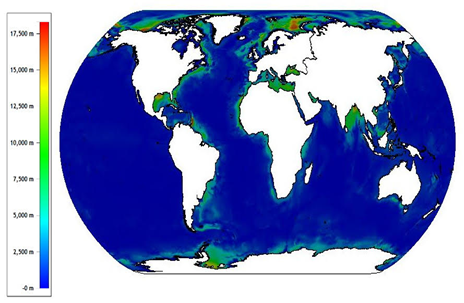
Figure 1. Depth to basement of marine sediments from Straume et al. (2019).

 

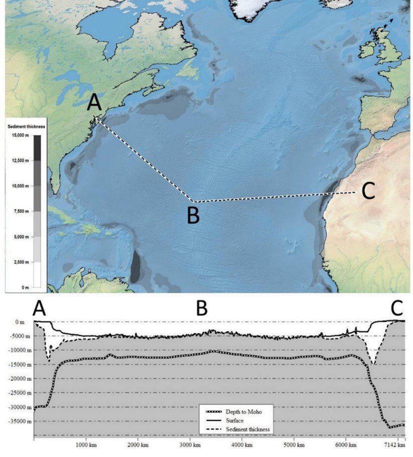
Figure 2. Cross section of Atlantic Ocean showing very thick sediments on the margins and the depth to the top mantle (Moho). Note deep troughs along the margins of North America and Africa (Straume et al., 2019).

 

 

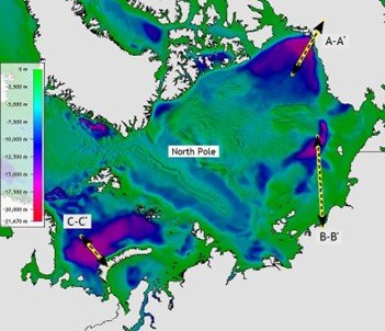
Figure 3. Sediment thickness of the Arctic Ocean (Straume et al., 2019).

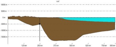
Figure 4. Line A-A´ from Figure 3 (Straume et al., 2019). Blue is ocean and brown is sediments. This same color scheme is used for the other cross sections. Vertical line shows the shoreline.

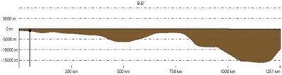
Figure 5. Line B-B´ from Figure 3 (Straume et al., 2019). Note that the continental shelf is so shallow that the blue ocean is not visible.

 

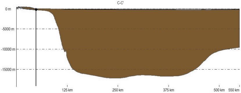
Figure 6. Line C-C´ from Figure 3 (Straume et al., 2019). Note that the continental shelf is so shallow that the blue ocean is not visible.

 

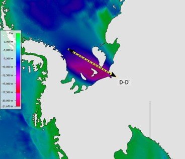
Figure 7. Sediment thickness of the Weddell Sea, Antarctica (Straume et al., 2019).

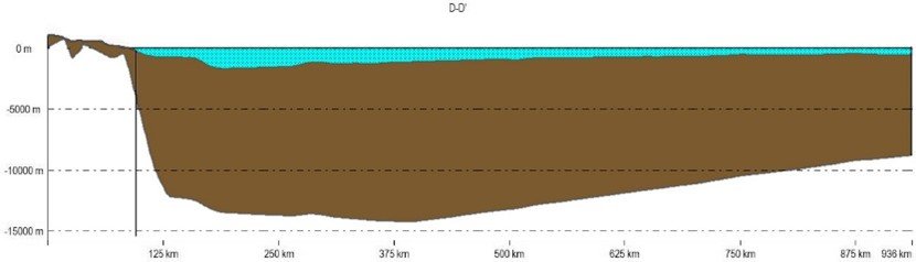
Figure 8. Line D-D´ from Figure 7 in the Weddell Sea, off Antarctica (Straume et al., 2019). Note that shelf depth increases landward, due to the weight of Antarctic Ice Sheet.

 

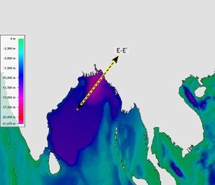
Figure 9. Sediment thickness in the Bay of Bengal (Straume et al., 2019).

 

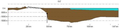
Figure 10. Line E-E´ from Figure 9 (Straume et al., 2019).

 

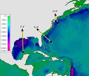
Figure 11. Sediment thickness off southeast United States (Straume et al., 2019).

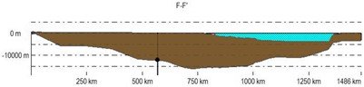
Figure 12. Line F-F´ from Figure 11 (Straume et al., 2019).

 

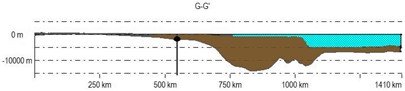
Figure 13. Line G-G´ from Figure 11 (Straume et al., 2019).

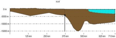
Figure 14. Line H-H´ from Figure 11 (Straume et al., 2019).

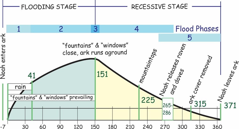
Figure 15. Timeline of the stages and phases of Flood from the Bible using Walker's (1994) Biblical geological model.

 

Possible Sources of Ocean Sediments

There are six logical possibilities for the origin of the ocean sediments in Biblical Earth history (Figure 16A). These include: (1) existing pre-Flood sediments, (2) early-Flood marine sediments redeposited in a marine environment, (3) early-Flood continental sediments transported to marine settings, (4) late-Flood continental sediments transported to marine settings, (5) sediments generated by post-Flood catastrophes, or (6) sediments generated by post-Flood uniformitarian processes (rivers, wind, ice). The Ice Age was not one of these uniformitarian processes, but will be included with number 6.

 

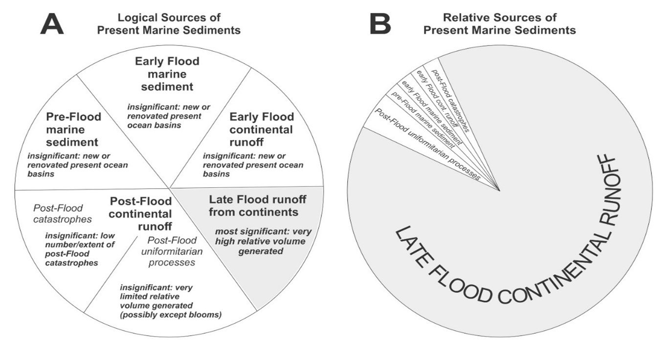
Figure 16. Potential logical sources of present marine sediment (A) and after assessing for their volumetric contributions (B). The vast bulk of actual sediments are best attributed to late-Flood continental runoff. Volume of minor components are exaggerated at right to allow room for text.

The first three options at the top half of Figure 16A-pre-Flood and early Flood continental and marine sediments-are rendered insignificant by the mid-Flood realignment of continents and ocean basins (Psalm 104), which would have minimized their contribution, either because the relative volume was low or because they were eroded and redeposited on the present continents or accreted on to the edge of the continents as metamorphic terranes. And if CPT is correct, many of these sediments would have been destroyed by subduction processes. The very low volume of deep-marine sediment supports this conclusion. The other three options at the bottom of figure 16A-late Flood runoff and post-Flood catastrophic or uniformitarian deposition will be evaluated below.

Did Post-Flood Catastrophes Occur?

Post-Flood catastrophes are one of the possible sources of ocean sediments shown at the bottom of Figure 16A. The magnitude of these possible post-Flood catastrophes can be determined mainly by Cenozoic history. The Flood/post-Flood boundary, whether at or near the K/Pg boundary or in the late Cenozoic (Miocene, Pliocene, or Quaternary [1] ) depending upon location (Oard, 2022a), has been extensively examined and debated. Oard (2014a, 2016, 2017a, 2017b, 2018, 2019) developed 33 criteria (Table II) supporting a Late Cenozoic boundary. Any one criterion may be equivocal, which is why multiple criteria are required to determine the boundary at a particular location. Clarey (2017, 2020) reinforced several of these criteria and added two additional lines of evidence not mentioned by Oard: (1) the early Cenozoic Whopper Sand is thick and widespread in the Gulf of Mexico, pointing to large, powerful currents well out into the Gulf, and (2) traditional landing site for the Ark in Turkey is surrounded by uninterrupted Cenozoic marine strata (Clarey and Werner, 2019). Both are readily explained by the Flood but inexplicable by post-Flood catastrophes. Tomkins and Clarey (2022) have further marked the boundary as near or at the Neogene/Pleistocene boundary.

Despite Oard and Clarey presenting 35 criteria for a late Cenozoic Flood/post-Flood boundary, Ross (2012) and Arment (2020) hold that the boundary is at or just above the K/Pg boundary-based primarily on only one criterion, fossil data. They have not examined the 35 criteria and presented alternative mechanisms supporting their placement of the Flood/post-Flood boundary. But, the lead author has examined the fossil arguments (Oard, 2022b, 2022d). He found that Australian marsupials, dated as old as late Oligocene, were at first dated as Pleistocene, which would be expected in Biblical Earth history. And then later, paleontologists found "primitive" features in some marsupials and gradually pushed back the dates, finally ending in the late Oligocene, based on the "stage of evolution." Oard (2022b) has argued these marsupials are post-Flood, agreeing with Arment, and explained them by rafting on log/vegetation mats into Australia early in the Ice Age (Oard, 2022c). In this case, the Flood/post-Flood boundary is in late Oligocene, but only at those limited unique fossil locations. Oard (2022d) also discovered that Ross's (2012) North American mammal arguments are equivocal in that many mammals, supposed to be unique to only North America, are not unique to North America. Some North American Pleistocene (assumed post-Flood by Oard) and some Tertiary mammals (assumed from the Flood by Oard) are also found on other continents. Moreover, Ross and Arment have not demonstrated that the "defined genera" they claimed that crossed the Flood/post-Flood boundary, as believed by Oard, are precisely the same and not just similar. Why can't there be similar genera and families within a Genesis kind existing both before and after the Flood?

Some creation scientists have suggested hypercanes as causing post-Flood catastrophes. Hypercanes are hypothetical super hurricanes generated over water temperatures around 40°C or greater that generate concentrated areas of heavy rainfall for erosion. Just like hurricanes, hypercanes take time to develop, so the initial storm must intensify slowly over a hot water source hundreds of kilometers wide, possibly generated by hot ocean-bottom rocks. So, both the atmosphere and water must almost be at rest to generate hypercanes. Moreover, hypercanes can only produce a limited amount of rain caused by moisture input into the storm, and once they move over land, they weaken fast. Hypercanes are unlikely after the Flood, and if they occurred would not be significant enough to produce huge post-Flood catastrophes as deduced from Cenozoic history.

The Flood Regression Model concludes that the Flood/post-Flood boundary is in the Late Cenozoic and proposes that the boundary is especially geomorphological, with two conjoined sets of landforms created by upstream erosion and downstream deposition. Upstream are large planation surfaces, erosional remnants (inselbergs), and long transported resistant rocks formed by the Sheet Flow Phase 4 (Figure 15). The subsequent Channelized Flow Phase 5, produced more linear to localized landforms, such as valleys, canyons, water and wind gaps, and pediments. Downstream are vast continental margin sedimentary wedges from continental erosion, with planar upper surfaces formed during the Sheet Flow Phase. These were incised by channels of various scales during the Channelized Flow Phase forming deep submarine canyons. Both upstream and downstream features show decreasing energy over time as currents narrowed with time and are only superficially modified by comparatively low-energy, present-day rivers, currents, storms, and slumps.

 

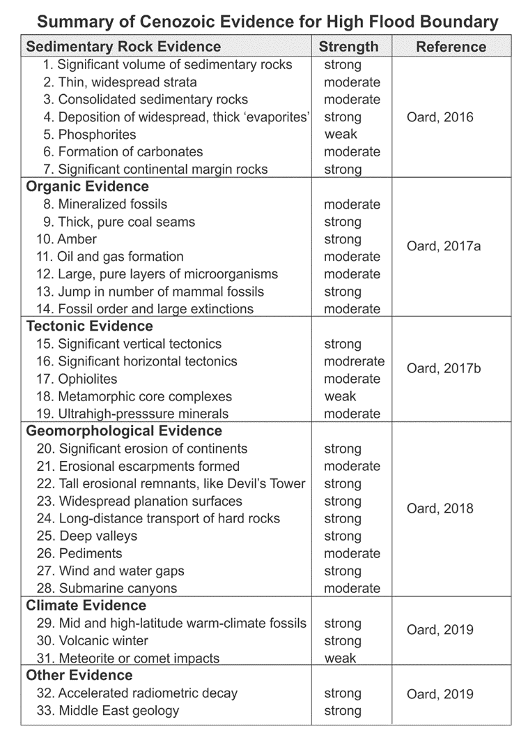
Table II. Evidence for a late Cenozoic boundary. Relative strength refers to the difficulty for a K/Pg boundary explanation.

 

 

Uniformitarian Marine Sediment Sources Since the Flood

Uniformitarian sediment sources after the Flood are a second possible source of ocean sediments shown at the bottom of Figure 16A. Sediments are transported by water, wind, ice, and volcanic eruptions or are authigenic: chemical and biogenic. The direct precipitation of chemicals, carbonates, and evaporites, limited to specialized environments, is relatively insignificant. Microorganism blooms, on the other hand, supply the water column with a steady rain of carbonaceous and siliceous skeletons. Most dissolve in the deep ocean, but some accumulate on the bottom as carbonaceous or siliceous oozes.

Sediment Added from Continental Erosion

Continents supply clastic sediment primarily through rivers today. To estimate the volume from rivers and streams since the Flood, we use Roth's (1998, p. 263) estimate that the continental erosion rate is 61 mm/ka. Applying strict actualism, the average depth eroded during 4500 years would be only 0.275 m. The area of the oceans is 3.61 x 10⁸ km ²; the continents is 1.49 x 10⁸ km². So, the 0.275 m would be dispersed over 2.4 times the source area, resulting in 0.115 m of marine sediment, mostly added to the continental margins. Higher Ice Age erosion would have increased this amount, but even an order of magnitude increase would be nothing compared to the oceanic average 975 m or the 3044 m average of the continental margins.

Sediment Added by Wind

Dust blown from deserts supplies some marine sediments (Froede, 2003). It is estimated that the Sahara Desert supplies 70% of the total annual dust input-800 Tg (teragrams) (Prospero and Mayol-Bracero, 2013). This works out to 0.062 km³/yr. or 279 km³ since Flood, which is also insignificant.

Ice Age dust contributions would probably not have been much greater because of the wet global climate in the early- to mid-Ice Age (Oard, in press). More dust would have originated from eastern Asia, Australia, and southern South America, but only at the end and after the Ice Age, when conditions become drier and windier (Oard, in press). The contribution from the Sahara Desert would have been less, since it was not a desert until well after the Ice Age (Oard, 2021).

Sediment Added by Ice and Volcanism

The amount of sediment added since the Ice Age by ice and volcanism is expected to be small. This input may have been more significant immediately after the Flood, since volcanism was high compared to the present, but we would expect the relative contribution to also be small compared to the total.

A recent estimate of the proportion of sediments added by ice and wind to the oceans today is approximately 20% of the river flux (Regard et al., 2022), which justifies our assumption that this input is small. The amount of sediment added to the oceans by coastal cliff erosion has been estimated to be only 2-4%. However, the researchers were surprised that coastal cliff erosion in Europe amounts to about 33% of the river flux. Regardless, this amount is small for our purposes.

Therefore, we have determined that practically all the margin sediments are from continental erosion during Flood runoff (Figure 16B). This volume and thickness represents erosion of 1500 m of sediment from the continents.

The Oceanic Microorganism Source

The largest potential source of post-Flood marine sediment comes from microorganism skeletons. At the present rate of accumulation of 1-3 cm/1000 years for carbonate skeletons (Kennett, 1982), deposition over 4500 years would be only 0.01 m. The deposition by siliceous organisms, such as diatoms and radiolarians, is probably similar but more important in the deep ocean.

However, the volume was likely much greater in the Ice Age, given the great vertical overturning of the oceans from cooling of the new, warm oceans from the top down (Oard, in press). Water near the surface was cooled by evaporation and contact with a cooler atmosphere. It sank, forcing warmer, deeper water to the surface. Since nutrients tend to collect in the deep ocean, a strong vertical overturn would have brought them to the surface layers, resulting in massive blooms and concomitant deposition of their skeletons.

Therefore, some part of the 404 m-average sediment thickness of the deep-sea floor could have occurred after the Flood. We do not know the relative contributions because no creation scientist has examined the ocean sediments in detail. We do not trust evolutionary dates of microorganisms, mostly calculated by biostratigraphy. More investigation is required.

In order to determine the amount of microorganisms and other sediments added to the deep ocean, we calculate a range of possibilities (left-hand side of Table III). There are five options, depending upon what percentage of the deep-sea sediments are from the Flood. The range is from none of the deep-sea sediment (0%) is from the Flood to all of it (100%) is from the Flood. The right side of Table III is the corresponding depth of eroded sediment during Flood recession by adding the possible proportions of deep-sea Flood sediments to 1500 m. At this point, we will arbitrarily use 50% of the deep-ocean sediments from the Flood with an average depth of 1886 m eroded from the continents.

Percent of Deep-Ocean Sediment from Flood	Depth Eroded from the Continents
0% (0 km3)	1500 m
25% (0.28 x 108 km3)	1692 m
50% (0. 57 x 108 km3)	1886 m
75% (0.85 x 108 km3)	2074 m
100% (1.13 x 108 km3)	2262 m

Table III. Five estimates of percent of deep-ocean sediments from the Flood and the corresponding average depth of erosion from the continents. We assumed that all the sediment from the margin and the area between the margin and the deep-ocean sediments, 2.24 x 10 ⁸ km³, are from Flood runoff. The area of the continents is 1.49 x 10⁸ km² and placing this sediment back on the continents results in erosion of 1500 m.

 

Strong Differential Vertical Tectonics

During the Recessive Stage, sediment was transported from continents by strong currents and deposited in velocity traps created by a dramatic depth change at the continent/ocean boundary (Figure 17). These deepening ocean margins provided significant accommodation space, keeping sediments predominantly at the margins, instead of spreading to the abyssal plains. We call this Differential Vertical Tectonics (DVT), which means that part of the continents rose, the ocean basins sank, or both.

DVT was especially prominent along the continental margins. For whatever reason, the eastern United States underwent many km of DVT, generating significant potential energy (Figure 2). Pazzaglia and Gardner (1994) describe this DVT as epeirogenic uplift of the Appalachian Piedmont and subsidence of the offshore area. Early in the Recessive Stage, the Floodwater rushed over and off the Appalachians, eroding up to 6 km (Oard, 2013, Appendix 4). Resulting debris was rapidly transported east and deposited in a seaward-prograding wedge, as the margin sank. As the Flood water level dropped on the continents, erosion and deposition migrated downgradient.

Current strength can possibly be retrodicted, as conditions of water volume, current width, gradient, depth, etc., are approximated, first using present topography. These estimates can be checked against the volume and geometry of the downgradient sediment wedge, particularly where it requires broad sheet-like currents early in the event.

During the Flood runoff, some sediment would have likely continued out onto the abyssal plains, where it first preferentially filled lows in the rough igneous basement. Downslope debris flows may have helped transport some sand onto the abyssal plain. This continues today via slides off the continental slope. Turbidity currents can be initiated by submarine landslides and travel on nearly flat slopes. Figure 17 is a schematic of the Flood formation of the continental margin off southeast Africa.

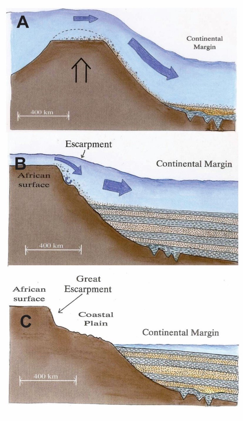
Figure 17. Flood formation of the continental margin off southeast Africa (drawn by Melanie Richard).

The vast majority of marine margin sediments was deposited as water velocity dropped. Water draining into those new oceans generated upgradient erosion and downgradient deposition, forming the time-transgressive post-Flood boundary, from upgradient planation surfaces to downgradient sediment wedges. The average erosion of the continents was estimated at about 1900 m, which is about 280,000,000 km³. We shall round off to 2000 m.

How Much Sediment at the Peak of the Flood?

 

We can add the amount of sediment eroded during the Recessive Stage of the Flood to the sedimentary rocks left on the continent to determine the amount of sediments piled on the continent at the peak of the Flood. Since we do not know the average sedimentary rock thickness left on the continents at the beginning of Flood runoff, we are calculating the average depth for various states of the United States. In the results so far, we estimate as a first guess about 2000 m. If about 2000 m was eroded off during Flood runoff and about 2000 m is left, then the total sediment thickness at the peak of the Flood was around 4000 m (Figure 18).

Most commentators believe that the peak of the Flood was reached on Day 150 (Boyd and Snelling, 2014; Johnson and Clarey, 2021). If our estimates of erosion and deposition are correct, then an approximate average of 4000 m of sediment existed at that time on the present-day continents. That is an average of more than 25 m of deposition per day. Since activity would have been greater at particular places and times, and less at other places at other times, the maximum volume deposited on any given day in any given location would have been much greater. But this is not surprising. The scale of processes taking place was unprecedented and unique. Analogies help us understand how great it might have been. For example, the Lake Missoula Flood eroded 125 km³ of soft silt and hard basalt in several days (Oard, 2004, 2014b). Deposition in some of the tributary valleys of eastern Washington was likely several meters per hour. We know that large-scale, energetic processes accomplish significant geological work. Now, we are starting to reach a point where we can constrain and begin to understand the scale of processes during the Flood.

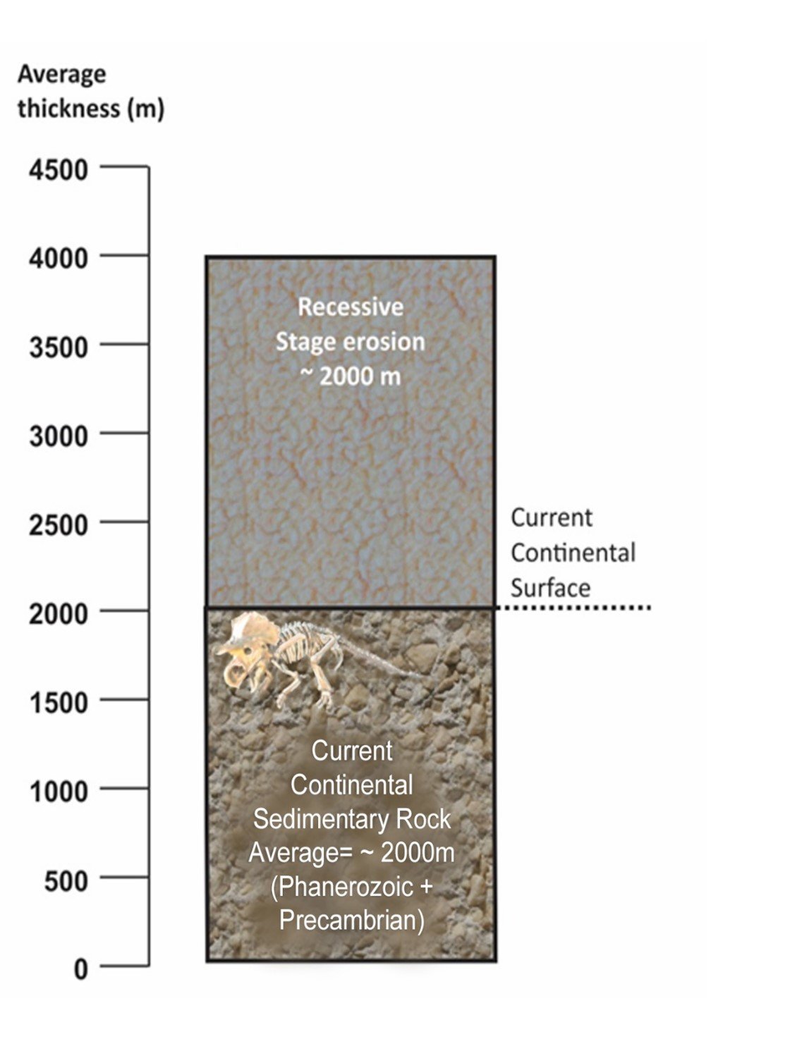
Figure 18. A block diagram representing the sediments and sedimentary rocks at Day 150 made up of about 50% remaining continental sediments and 50% that has been eroded during the Recessive Stage (modified by Mrs. Melanie Richard).

 

Geomorphological Features Contrary to Uniformitarianism

Many geomorphological features resulting from a Flood Regression Model confound uniformitarians because modern processes would never create them (Oard, 2013). Following, are a few examples.

Sediments Carried off the Continents

Slow, gradual erosion over millions of years would have resulted in massive flood plains on the continents, the residue of lower-energy processes. However, we see planation surfaces that generated large volumes of sediment, not deposited on the continents, but along the continent-ocean margin. Powerful currents would have been required to erode the estimated 1900 m of sediment off the continents.

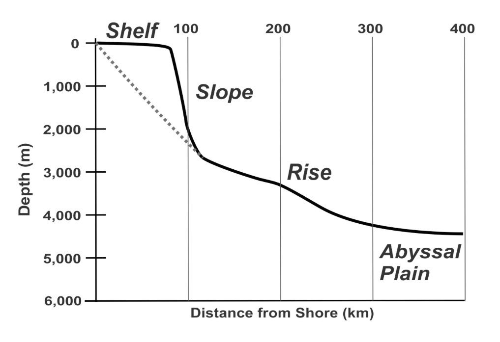
Figure 19. Profile of continental margin off Cape Hatteras, North Carolina, exhibiting classic shelf-slope-rise architecture. Modified from Sauter (2004). Vertical exaggeration = 50x.

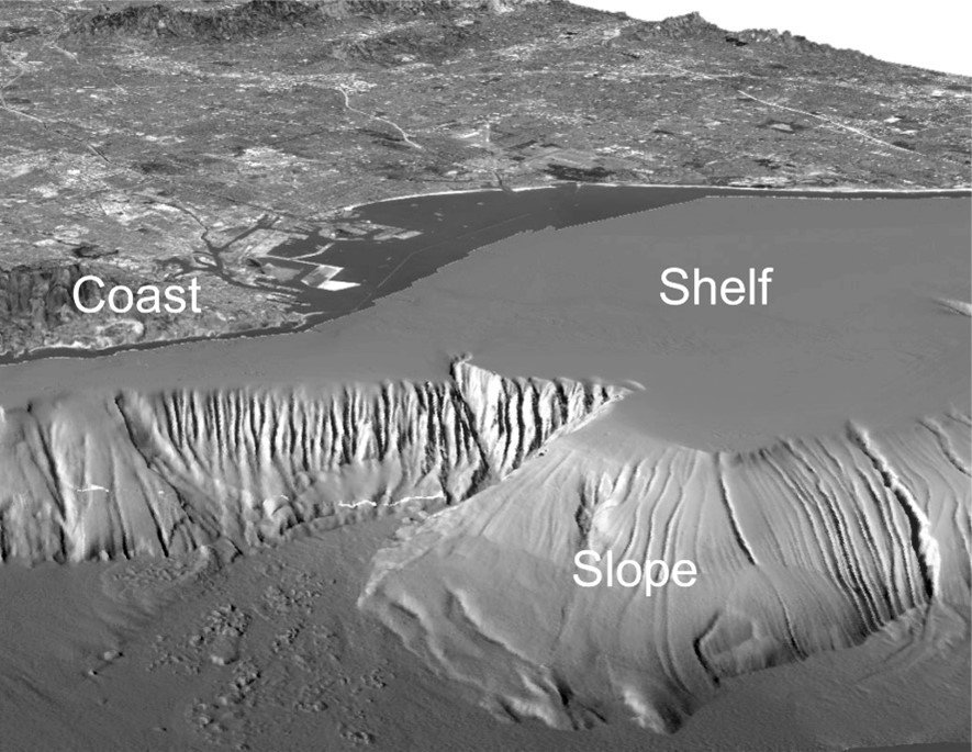
Figure 20. Continental shelf and slope near Los Angeles, California, showing dramatic geomorphology hidden underwater. Modified from USGS Coastal and Marine Hazards and Resources Program Decadal Strategic Plan, 2020-2030 .

Continental Margin Profiles Look Young

Continental margins do not steadily drop in elevation from the shore. Instead, they create the distinct profile of the shelf, slope, and rise (Figure 19). The continental shelf is a seaward extension of the coastal plain to the shelf break or shelf edge, which marks the beginning of the continental slope. The continental shelf dips very gently-less than 0.1° and widths vary; the average is 80 km. At least one shelf is over 1,000 km wide (Hedberg, 1970). The widest shelves are found along the Arctic Ocean, in the Bering Sea, and the Grand Banks, off Newfoundland.

 

Continental shelves break at a consistent average depth of about 130 m, except off Antarctica where ice has depressed the shelf. Beyond the shelf break, the surface slopes seaward at about 4°, from 130 m to 1500-3500 m. Slopes vary: some reach 35° to 90°. Slope widths are narrow compared to shelves. Slope topography changes more rapidly: faulting, submarine slides, and submarine canyons leave their imprint. Yet the slope is majestic. If water were removed from the oceans, the continental slope would be the most conspicuous geomorphological boundary on Earth (Figure 20). No one knows why the shelf-slope break occurs at 130 m, but its global consistency suggests the synchronous end of the Flood. Otherwise, deposition of the margins would be more chaotic. It could simply be the type of crust beneath the continent and the ocean causing the relief.

Extensive continental rises exist only along passive margins with no offshore deep-sea trench. Rises show a gradual decline in slope seaward of the continental slope and provide the transition down to the deep abyssal plains. The rise can vary from 100-1,000 km wide with a much lower relief than the slope.

Though few uniformitarians address it, the continental margin profile is unexpected, if they are really millions of years old as claimed. Present processes, over time, would favor a gradual slope from continents to deep ocean (the dashed line on Figure 19). King (1983, p. 199), described the problem:

There arises, however, the question as to what marine agency was responsible for the leveling of the shelf in early Cenozoic time, a leveling that was preserved, with minor modification, until the offshore canyon cutting of Quaternary time? Briefly the shelf is too wide, and towards the outer edge too deep, to have been controlled by normal wind-generated waves of the ocean surface (emphasis mine).

When King wrote, it was believed that submarine canyons were Quaternary, but uniformitarian scientists have pushed the origin of submarine canyons well down into the Cenozoic. King implies that present processes cannot form the existing margin profile because winds generate most ocean currents (Wunch, 2006) and resulting currents, e.g., the Gulf Stream, run parallel to the coast (Kennett, 1982). Continental sediments are moved to the margins by rivers and their deltas, which show seaward, nearly-flat progradation to a slope break. Longshore currents and storms spread the sediments along the continental margins. Sediments are transported into deep water by slumping and other mass movements, ubiquitous along the continental slopes today. Such slumping over deep time would create a more gradual profile (dashed line in Figure 19.)

Thus, the continental shelf and slope are like a giant delta, occupying continental margins. Such continental scale bodies were formed by water flowing off the continents in "rivers" thousands of km wide.

A small-scale example is the delta of the Colorado River at Lake Mead, in the narrow Lower Granite Gorge (Figure 21), that formed as the lake filled. There were no longshore currents to spread the sediment, which was deposited in a narrow gorge. The top of the delta is nearly flat until it reaches a steep drop off. This example sheds light on the formation of the continental shelf and slope by wide, Flood sheet currents.

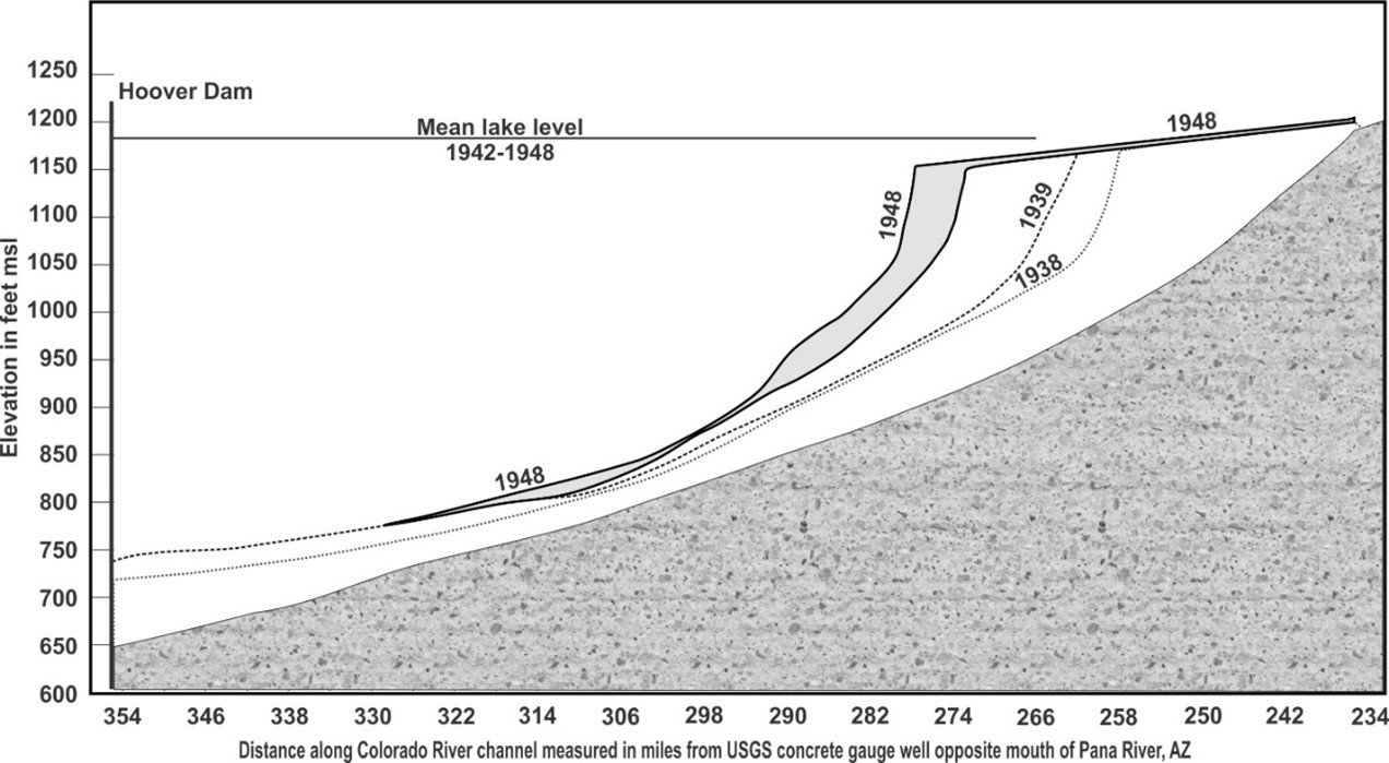
Figure 21. The yearly prograding Colorado River delta into Lake Mead in the Lower Granite Gorge as the lake was filling (modified by Mrs. Melanie Richard). There could be no lateral movement of the sediments, like in ocean deltas today, providing a schematic of the formation of the continental shelf and slope by offshore sheet currents during Flood runoff.

 

Summary and Future Directions

A Flood Regression Model seeks to understand processes associated with the vertical restructuring of Earth's crust into its present configuration. Of particular interest is the linked triad of erosion, transport, and deposition of sediments off the continents and mostly onto the continental margins.

Determining a stratigraphically high post-Flood boundary from 35 criteria and post-Flood uniformitarian processes that deposit very little sediment in the oceans, we conclude that most marine sediments are the products of the Recessional Stage of the Flood. We seek to describe and understand specific processes of: (1) DVT as it relates to erosion, transport, and deposition; (2) the nature of the post-Flood boundary as a time-transgressive geomorphological boundary; (3) the extent of erosion off the continents and its implications for earlier Flood conditions; and (4) the manner of deposition of that sediment in broad, prograding sheets at the margins. The margin deposition was aided by rapidly deepening ocean basins needed to create velocity traps for the sediment. We estimate an average continental thickness of ~2000 m was deposited mainly at the margins (Figure 1).

---

Figures

Figure 1. Depth to basement of marine sediments, a general measure of sediment thickness (from Straume et al., 2019).

 

Figure 2. Cross section of Atlantic Ocean showing very thick sediments on the margins and the depth to the Moho. Note deep troughs along the margins of North America and Africa (from Straume et al., 2019).

 

Figure 3. Sediment thickness of the Arctic Ocean (from Straume et al., 2019).

 

Figure 4. Line A-A´ from Figure 3 (from Straume et al., 2019). Blue is ocean and brown is sediments. This same color scheme is used for the other cross sections. Vertical line shows the shoreline.

 

Figure 5. Line B-B´ from Figure 3 (from Straume et al., 2019). Note that the continental shelf is so shallow that the blue ocean is not visible.

 

Figure 6. Line C-C´ from Figure 3 (from Straume et al., 2019). Note that the continental shelf is so shallow that the blue ocean is not visible.

 

Figure 7. Sediment thickness of the Weddell Sea, Antarctica (from Straume et al., 2019).

 

Figure 8. Line D-D´ from Figure 7 in the Weddell Sea, off Antarctica (from Straume et al., 2019). Note that shelf depth increases landward, due to the weight of Antarctic Ice Sheet.

 

Figure 9. Sediment thickness in the Bay of Bengal (from Straume et al., 2019).

 

Figure 10. Line E-E´ from Figure 9 (from Straume et al., 2019).

 

Figure 11. Sediment thickness off southeast United States (from Straume et al., 2019).

 

Figure 12. Line F-F´ from Figure 11 (from Straume et al., 2019).

 

Figure 13. Line G-G´ from Figure 11 (from Straume et al., 2019).

 

Figure 14. Line H-H´ from Figure 11 (from Straume et al., 2019).

 

Figure 15. Timeline of the stages and phases of Flood from the Bible using Walker's (1994) Biblical geological model.

 

Figure 16. If potential logical sources of present marine sediment (A) are assessed for their volumetric contributions (B), it becomes clear that the vast bulk of actual sediments are best attributed to late-Flood runoff. Volume of minor components are exaggerated at right to allow room for text.

 

Figure 17. Flood formation of the continental margin off southeast Africa (drawn by Melanie Richard).

 

Figure 18. A block diagram representing the sediments and sedimentary rocks at Day 150 made up of about 50% remaining continental sediments and 50% that has been eroded during the Recessive Stage ( modified by Mrs. Melanie Richard ).

 

Figure 19. Profile of continental margin off Cape Hatteras, North Carolina, exhibiting classic shelf-slope-rise architecture. Modified from Sauter (2004). Vertical exaggeration = 50x.

 

Figure 20. Continental shelf and slope near Los Angeles, California, showing dramatic geomorphology hidden underwater. Modified from USGS Coastal and Marine Hazards and Resources Program Decadal Strategic Plan, 2020-2030 .

 

Figure 21. The yearly prograding Colorado River delta into Lake Mead in the Lower Granite Gorge as the lake was filling (modified by Mrs. Melanie Richard). There could be no lateral movement of the sediments, providing a schematic of the formation of the continental shelf and slope by offshore sheet currents during Flood runoff.

 

 

---

References

CRSQ : Creation Research Society Quarterly

NOAA : National Oceanic and Atmospheric Administration

>Arment, C. 2020. To the Ark, and back again? Using the marsupial fossil record to investigate the post-Flood boundary. Answers Research Journal 13: 1-22.

Barrick, W., M.J. Oard, and P. Price. 2020. Psalm 104:6-9 likely refers to Noah's Flood. Journal of Creation 34(1): 102-109.

Barrick, W.D. 2018. Exegetical analysis of Psalm 104:8 and its possible implications for interpreting the geologic record. In Whitmore, J.H. (editor), Proceedings of the Eight International Conference on Creationism, pp. 95-102. Creation Science Fellowship, Pittsburgh, PA.

Boyd, S.W., and Snelling, A.A. (editors). 2014. Grappling with the Chronology of the Genesis Flood. Master Books, Green Forest, AR.

Chardon, D., V. Chevillotte, A. Beauvais, G. Grandin, and B. Boulangé. 2006. Planation, bauxites and epeirogeny: One or two palaeosurfaces on the West African margin? Geomorphology 82: 273-282.

Clarey, T. 2020. Carved in Stone: Geological Evidence of the Worldwide Flood. Institute for Creation Research, Dallas, TX.

Clarey, T.L. 2017. Local catastrophes or receding Floodwater? Global geologic data that refute a K-Pg (K-T) Flood/post-Flood boundary. CRSQ 54(2): 100-120.

Clarey, T.L., and D.J. Werner. 2019. Compelling evidence for an Upper Cenozoic Flood/post-Flood boundary: Paleogene and Neogene marine strata that completely surround Turkey. CRSQ 56(2): 68-75.

Ducea, M.N., and J.B. Saleeby. 1996. Buoyancy sources for a large, unrooted mountain range, the Sierra Nevada, California: Evidence from xenolith thermobarometry. Journal of Geophysical Research 101(B4): 8229-8244.

Eaton, D.W., F. Darbyshire, R.L. Evans, H. Grütter, A.G. Jones, and X. Yuan. 2009. The elusive lithosphere-asthenosphere boundary (LAB) beneath cratons. Lithos 109: 1-22.

Eaton, G.P. 2008. Epeirogeny in the Southern Rocky Mountains region: Evidence and origin. Geosphere 4(5): 764-784.

Froede Jr., C.R. 2003. Dust storms from the sub-Saharan African continent: Implications for plant and insect dispersion in the post-Flood world. CRSQ 39(4): 237-244.

Gansser, A. 1964. Geology of the Himalayas. Interscience Publishers, New York, NY.

Hedberg, H.D. 1970. Continental margins from viewpoint of the petroleum geologist. AAPG Bulletin 54(1): 3-43.

Ivany, L.C., S. Van Simaeys, E.W. Domack, and S.C. Sampson. 2006. Evidence for an earliest Oligocene ice sheet on the Antarctic Peninsula. Geology 34(5): 377-380.

Johnson, J.J.S., and T.L. Clarey. 2021. God floods Earth, yet preserves Ark-borne humans and animals: Exegetical and geological notes on Genesis Chapter 7. CRSQ 57(4): 248-262.

Karl, H.A., P.R. Carlson, and J.V. Gardner. 1996. Aleutian basin of the Bering Sea: Styles of sedimentation and canyon development. In Gardner, J.V., M.E. Field, and D.C. Twichell (editors), Geology of the United States' Seafloor-The View from GLORIA, pp. 305-332. Cambridge University Press, New York, NY.

Kennett, J. 1982. Marine Geology. Prentice-Hall, Englewood Cliffs, NJ.

King, L.C. 1982. The Natal Monocline, second revised edition. University of Natal Press, Pietermaritzburg, South Africa.

King, L.C. 1983. Wandering Continents and Spreading Sea Floors on an Expanding Earth . John Wiley and Sons, New York, NY.

Klevberg, P., and M. Oard. 1998. Paleohydrology of the Cypress Hills Formation and Flaxville Gravel. In Walsh, R.E. (editor), Proceedings of the Fourth International Conference on Creationism , technical symposium sessions, pp. 361-378. Creation Science Fellowship, Pittsburgh, PA.

Love, J.D. 1960. Cenozoic sedimentation and crustal movement in Wyoming. American Journal of Science 258-A: 204-214.

Macdonald, K.C., P.J. Fox, R.T. Alexander, R. Pockalny, and P. Gente. 1996. Volcanic growth faults and the origin of Pacific abyssal hills. Nature 380: 125-129.

Mintz, Y. 1968. Very long-term global integration of the primitive equations of atmospheric motion: An experiment in climate simulation. In Mitchell, Jr., J.M. (editor), Causes of Climate Change, Meteorological Monographs. Volume 8, Number 30, pp. 20-36. American Meteorological Society, Boston, MA.

Oard, M.J. 2004. The Missoula Flood Controversy and the Genesis Flood. Creation Research Society Books, Glendale, AZ.

Oard, M.J. 2011a. The remarkable African planation surface. Journal of Creation 25(1): 111-122; https://creation.com/african-planation-surface .

Oard, M.J. 2011b. Retreating Stage formation of gravel sheets in south-central Asia. Journal of Creation 25(3): 68-73; https://creation.com/south-asia-erosion .

Oard, M.J. (ebook). 2013. Earth's Surface Shaped by Genesis Flood Runoff, http://Michael.oards.net/GenesisFloodRunoff.htm .

Oard, M.J. (ebook). 2014a. The Flood/Post-Flood Boundary Is in the Late Cenozoic with Little Post-Flood Catastrophism . http:// Michael.oards.net/PostFloodBoundary.htm .

Oard, M.J. 2014b (DVD). The Great Missoula Flood: Modern Day Evidence for the Worldwide Flood . Awesome Science Media, Richfield, WA.

Oard, M.J. 2016. Flood processes into the late Cenozoic-sedimentary rock evidence. Journal of Creation 30(2): 67-75.

Oard, M.J. 2017a. Flood processes into the late Cenozoic: part 3-organic evidence. Journal of Creation 31(1): 51-57.

Oard, M.J. 2017b. Flood processes into the late Cenozoic: part 4-tectonic evidence. Journal of Creation 31(1): 58-65.

Oard, M.J. 2018. Flood processes into the late Cenozoic: part 5-geomorphological evidence. Journal of Creation 32(2): 70-78.

Oard, M.J. 2019. Flood processes into the late Cenozoic: part 6-climatic and other evidence. Journal of Creation 33(1): 63-70.

Oard, M.J. 2021. Ice core oscillations and abrupt climate changes: part 5-the early Holocene green Sahara. Journal of Creation 35(3): 103-108.

Oard, M.J. 2022a. Does paleontology nullify geological arguments for the location of the Flood/post-Flood boundary? Setting the record straight. Journal of Creation 36(1): 81-88.

Oard, M.J. 2022b. Australian marsupials: There and back again? Journal of Creation 36(1): 99-106.

Oard, M.J. 2022c. When and how did the marsupials migrate to Australia? Journal of Creation 36(2): 90-96.

Oard, M.J. 2022d. Did post-Flood North American mammals live above their dead Flood relatives? Journal of Creation 36(3): 106-113.

Oard, M.J. (in press). The Great Ice Age: Only the Bible Explains It. Creation Book Publishers, Powder Springs, GA.

Oard, M., J. Hergenrather, and P. Klevberg. 2005. Flood transported quartzites-east of the Rocky Mountains. Journal of Creation 19(3): 76-90 ; https://creation.com/flood-transported-quartzites-part-1east-of-the-rocky-mountains .

Oard, M.J., J. Hergenrather, and P. Klevberg. 2006. Flood transported quartzites: Part 2-west of the Rocky Mountains. Journal of Creation 20(2): 71-81; https://creation.com/flood-transported-quartzites-part-2west-of-the-rocky-mountains .

Oard, M.J., and P. Klevberg. 1998. A diluvial interpretation of the Cypress Hills Formation, Flaxville gravel, and related deposits. In Walsh, R.E. (editor), Proceedings of the Fourth International Conference on Creationism , technical symposium sessions, pp. 421-436. Creation Science Fellowship, Pittsburgh, PA.

Ollier C., and C. Pain. 2000. The Origin of Mountains. Routledge, London, U.K.

Ollier, C.D., and C.F. Pain. 2019. Neotectonic mountain uplift and geomorphology. Journal of Geomorphology RAS 4: 3-26.

Pazzaglia, F.J., and T.W. Gardner. 1994. Late Cenozoic flexural deformation of the middle U.S. Atlantic passive margin. Journal of Geophysical Research 99 (B6): 12143-12157.

Pazzaglia, F.J., and T.W. Gardner. 2000. Late Cenozoic landscape evolution of the U.S. Atlantic passive margin: Insights into a North American Great Escarpment. In Summerfield, M.A. (editor), Geomorphology and Global Tectonics, pp. 283-302. John Wiley & Sons, New York, NY.

Pickering, K.T., R.N. Hiscott, and F.J. Hein. 1989. Deep-Marine Environments, pp. 263-269. Unwin Hyman, London, U.K.

Poag, C.W. 1992. U.S. middle Atlantic continental rise: Provenance, dispersal, and deposition of Jurassic to Quaternary sediments. In Poag, C.W., and P.C. de Graciansky (editors), Geological Evolution of Atlantic Continental Rises, pp. 100-156. Van Nostrand Reinhold, New York, NY.

Poag, C.W., and W.D. Savon. 1989. A record of Appalachian denudation in post-rift Mesozoic and Cenozoic sedimentary deposits of the U.S. middle Atlantic continental margin. Geomorphology 2: 119-157.

Prospero, J., and O.L. Mayol-Bracero. 2013. Understanding the transport and impact of African dust on the Caribbean Basin. Bulletin of the American Meteorological Society 94(9): 1329-1337.

Reed, J.K., M.J. Oard, and P. Klevberg. 2022. Where the sediments are. CRSQ 59(2): 103-110.

Regard, V., et al. 2022. Rock coast erosion: An overlooked source of sediments to the ocean. Europe as an example. Earth and Planetary Science Letters 579: 1-9.

Ross, M.J. 2012. Evaluating potential post-Flood boundaries with biostratigraphy-the Pliocene/Pleistocene boundary. Journal of Creation 26(2): 82-87.

Roth, A.A. 1998. Origins: Linking Science and Scripture. Review and Herald Publishing Association, Hagerstown, MD.

Sauter, L.R. 2004. A Profile of the Southeast U.S. Continental Margin. NOAA. https://oceanexplorer.noaa.gov/explorations/04etta/background/profile/profile.html

Straume, E.O., C. Gaina, S. Medvedev, K. Hochmuth, K. Gohl, J.M. Whittaker, R. Abdul Fattah, J.C. Doornenbal, and J.R. Hopper. 2019. Globsed: Updated total sediment thickness in the world's oceans. Geochemistry, Geophysics, Geosystems 10.1029/2018GC00815: 1756-1772.

Tomkins, J.P., and T. Clarey. 2022. Paleontology supports an N - Q Flood boundary. Acts & Facts 51(2): 7.

Walker, T. 1994. A Biblical geological model. In Walsh, R.E. (editor), Proceedings of the Third International Conference on Creationism , technical symposium sessions, pp. 581-592. Creation Science Fellowship, Pittsburgh, PA; biblicalgeology.net/ .

Wunsch, C. 2006. An oceanographer charts the ebb and flow of opinion on ocean currents. Nature 39: 513.

Footnotes

---