Towards a More Realistic Young-Earth Ice Sheet Model: A Shallow, Isothermal Ice Ridge with a Frozen Base

Towards a More Realistic Young-Earth Ice-Sheet Model: A Shallow, Isothermal Ice Ridge with a Frozen Base

Jake Hebert

Key Words: ice core, ice sheet, ice ridge, Larry Vardiman, M.W. Mahaffy, Ed Bueler, Ice Age, computer modeling, annual layer thicknesses

Introduction

Creation-based ice sheet models are still in their infancy. In 1993 Dr. Larry Vardiman of the Institute for Creation Research published an analytical model (Vardiman, 1993, 1994, and 2001) for the rapid formation of thick ice sheets within the 4500 years since the Genesis Flood. Vardiman's model assumed that post-Flood annual ice accumulation was very high immediately after the Flood and then decayed exponentially to today's "slow and gradual" values. It also implicitly assumed that the downward speed of the surface ice was proportional to the height of the ice sheet (Hebert, 2021, p. 179). As Vardiman noted, his effort was preliminary, and although this assumption simplified the mathematics, it was not completely physically realistic. Hence there is a need for improved creation-based ice sheet models to better compare and contrast creationist and uniformitarian ice sheet predictions.

Glaciologists have already devised ice-flow models which do not necessarily involve uniformitarian assumptions and which could conceivably be used to simulate the rapid growth of post-Flood ice sheets. One such model is the quasi-analytical ice-sheet model of M.W. Mahaffy, which he published in 1976. I have already used this model to simulate the growth of an isothermal ice dome in the 4500 years since the Genesis Flood (Hebert, 2022). This paper combines Vardiman's accumulation model with Mahaffy's ice sheet model to simulate the growth of a long (horizontal aspect ratio of 5:1) but relatively thin isothermal ice ridge.

The next sections provide a brief introduction to ice core basics and ice sheet modelling. These subjects are covered in much more depth in Bueler (2016) and Hebert (2021, 2022).

Ice Sheet Fundamentals

Glaciologists drill ice cores at ice divides, topographical "highs" named for the fact that ice on one side of the divide flows one way, and ice on the other side of the divide flows the other (Figure 1). For a perfectly flat surface, ice is deposited in perfectly horizontal layers. Assuming no shifting of the ice divide during buildup, ice at the divide will flow neither to the right nor left, but will move straight down as additional layers are added. It is also possible for the ice to form a dome around the divide, so that ice flows radially outward from the divide, not just right and left.

In fact, the azimuthally-symmetric ice dome is one of two simple, "archetypal" ice sheet geometries that can be modelled in just one horizontal dimension. The (infinitely) long ice ridge is the other (Paterson, 1980, pp. 19-24). The ice divides in Greenland are long and elongated (Anonymous), causing the two major Greenland ice domes to be elongated ridges (Paterson, 1980, p. 9). Hence this ridge geometry is also of interest. I have used the Mahaffy model to simulate the rapid post-Flood formation of an azimuthally-symmetric ice dome in a previous paper (Hebert, 2022). Here I use the Mahaffy model to simulate the rapid growth of a long (horizontal aspect ratio of 5:1) post-Flood ice ridge.

Ignoring possible isostatic adjustments, the underlying bedrock is locked in place. So a horizontal layer that reaches bedrock can no longer move downward, and its vertical velocity must be zero. Also, stresses on the ice layer thin the layer over time. If no melting occurs, the total number of true annual layers will equal the ice sheet's true age (in years). In that case, finding the average annual layer thickness is trivially easy: it is simply the height of the ice sheet divided by the number of years the ice sheet has been in existence. However, finding a particular layer thickness at a given depth is much more difficult, since the stresses that induce thinning vary with depth and time. Annual layers often consist of multiple visible bands. Creationists argue that uniformitarian glaciologists are mistaking visible bands for annual layers and are seriously overcounting the number of true annual layers within the ice cores (Oard 2005, 2006).

Ice sheet models typically ignore variations in ice density, which are tiny even for thick ice sheets (Cuffey and Paterson, 2010, pp. 12-13). Hence, most ice sheet models assume incompressibility, i.e., that the ice has a constant density (Paterson, 1980, p. 12; Cuffey and Paterson, 2010, p. 286). Glaciologists often use the letters u, v, and w to indicate ice velocities in the x, y, and z directions, respectively. The condition of constant density implies that the divergence of the velocity field is zero everywhere:

Although the volume of the ice sheet as a whole may increase via the deposition of additional ice, a particular layer of the ice sheet maintains a constant volume over time (assuming no melting or calving of the ice). Stresses cause the layer to thin, but with a corresponding increase in horizontal surface area so that the layer's volume remains constant.

Methods

The Mahaffy model

As noted earlier, Mahaffy's (1976) ice-sheet model does not assume the ice to be in steady state. It utilizes Glen's Flow Law (Glen, 1955; Nye, 1957; Paterson, 1980, pp. 13-16) and the assumption of incompressibility, and it effectively treats the ice as isothermal. Mahaffy's solution is obtained by solving the stress balance equations for a small parcel of ice. However, in order to simplify the mathematics, his model ignores normal stresses, as well as vertical shear stresses. In other words, he assumes that the ice sheet is deformed only by shear in the horizontal directions.

Mahaffy's model allows for non-level bedrock terrain, but here we make the simpler assumption that the bedrock under the ice is perfectly flat. We assume no melting at the base of the ice sheet, so the ice is frozen to the bedrock. Readers needing a refresher in the basics of ice sheet modeling may refer to Bueler (2016) and Hebert (2022).

Consider the generalized ice sheet depicted in Figure 2. The height of the ice h is a function of the horizontal coordinates x and y, as well as time t. We will use H = h (0, 0, t) to denote the height at the center of the ice sheet, i.e., the divide location.

Consider a thin column of ice of height h(x, y) and a square base with sides of length 1 meter (Figure 3). For the moment we ignore the horizontal motion of ice in the y direction. If u(z) is the (height-dependent) horizontal ice velocity in the x-direction, we may define q_x to be the volume of ice per unit length that flows horizontally (in the x-direction) into the vertical column in a time dt.

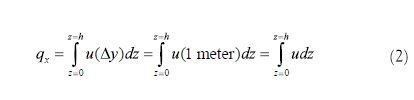
If q_x(x) equals q_x(x+1), so that q_x/= 0, there will be no net inflow or outflow of ice into the column (in the x direction), and, absent any additional ice deposition from above (as precipitation), the ice column's height will remain constant. If q_x(x+1) is greater than q_x(x), so that ∂q_x/∂x>0, there will be a net outflow of ice from the column, which will tend to cause the height of the ice column to decrease. Similarly, if there is a net inflow of ice into the column, causing the column height to increase.

Similar relationships hold for the y-direction. Hence, at a given location in the x-y plane, the height h(x, y, t) of the ice is governed by the continuity equation:

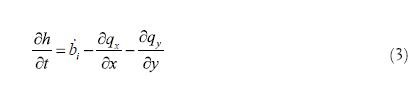
The net horizontal flow of ice into or out of the column will tend to change the height h, but so will the deposition of accumulating ice, indicated by b_i. In general, b_i is a function of both position (x, y) and time t and has units of meters of ice per year. After making some additional assumptions about the relative sizes of rates of change of the velocities relative to one another (which allowed some derivatives to be neglected), Mahaffy (1976) derived the following expressions (Paterson, 1980, p. 43) for the horizontal ice fluxes:

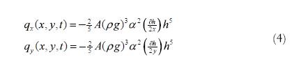[Text Wrapping Break]where

is the magnitude of the surface gradient. A is the temperature-dependent "softness" of the ice, ρ is the density of ice (910 kg/m³), and g is the acceleration due to gravity, 9.81 m/s². Details are provided in Mahaffy (1976) and Paterson (1980). If we define

we may combine Equations into a single expression for the flux vector q→:

Obtaining the solution

Bueler (2016) observes that we can express the continuity equation (3) in terms of the flux vector q→:

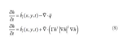
He then draws our attention to similarities between Equation (8) and the two-dimensional heat equation:

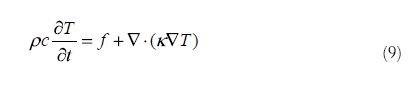
In Equation (9), f is the heat source term, ρ is density, κ is thermal conductivity, and c is specific heat. Dividing both sides of Equation (9) by ρc, the result has the same mathematical form as Equation (8):

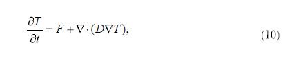
provided that we define D and F as

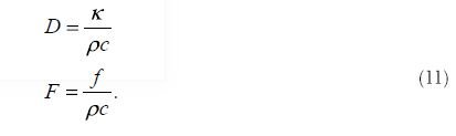
The choice of the letter D in Equation (10) is appropriate, since the heat equation is really a diffusion equation: a localized temperature "spike" will diffuse outward, with the peak becoming shorter and broader over time. Note that the same thing will be true for an ice peak. If we suppress any further deposition of ice, so that b_i=0, the already-deposited ice flows in such a way that a peak becomes shorter and broader over time, while the total ice volume remains constant. We can thus treat the flow of the ice as a diffusion problem if we define our position and time-dependent ice "diffusivity" to be

Bueler (2016) described how to solve Equation (8) using an explicit, finite difference solution with adaptive time-stepping, and he provided a sample MATHLAB code for doing so. I "translated" his code into an IDL code that I titled mahaffy_ridge_var_precip.pro, and I used my version to simulate the growth of a long isothermal ice ridge. Details and subtleties of the method are given in Bueler (2016).

Although the deposition and flow of ice is actually a continuous process, we must model it as a discrete two-step process. At the very beginning of a particular time step Δt, a layer of ice is instantaneously deposited. If Δt = 1 year, the entire year's total ice accumulation is deposited at the very start of the time interval. During the remainder of the time step, no more ice is deposited, but the already-deposited ice is allowed to flow/diffuse. At the beginning of the next time step, another layer of ice is instantaneously deposited. During the remainder of the second time step, the ice (now consisting of two deposited layers) is allowed to diffuse/flow some more. This deposit/diffuse process is repeated for the duration of the simulation.

It is worth noting that when a layer of ice is instantaneously deposited (at the very start of the time interval), it has no velocity at all, including no downward velocity w. Instead, the layer is instantaneously deposited, already "in place" as it were. Rather, the vertical velocity w refers to the velocity of the ice while it is in the process of diffusing during the remainder of the time interval.

Greenland accumulation rates

Accumulation rates may be expressed in several different ways. Sometimes it is expressed as b_i (meters or centimeters of ice equivalent per year). It may also be expressed as b_w (meters or centimeters of water equivalent per year) or as (grams per square centimeter per year). The relationships between these different expressions are (Cuffey and Paterson, 2010, p. 94):

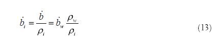
Oard (2005, pp. 2, 6) cites accumulation rates b_w reported by Ohmura and Reeh (1991) at the locations of major deep Greenland ice cores (GISP, GISP2, NGRIP) of between 20 and 24 centimeters of water equivalent per year. Using Equation and the densities of ice and water, this translates into about 22 to 26 centimeters of ice per year.

A more recent study (Bales et al., 2009) reported average Greenland accumulation rates b of about 30 g/cm²/year for the entire ice sheet, as well as for elevations above 2000 meters. This translates into an ice accumulation rate b_i of about 33 centimeters of ice per year. For this simulation, I used the more conservative value of b_i= τhλ = λ_H/τ = 24 cm/year = 0.24 meters of ice per year.

Results

Application of Vardiman's model

I used Vardiman's (1993, 1994, 2001) accumulation model

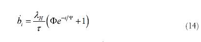
Vardiman used the symbol for his ice accumulation rate, but here I use to b_i be consistent with the notation already used above. The parameter Φ, used to "scale up" the amount of Ice Age precipitation compared to the present-day value, was set at 61.5. This resulted in an initial ice accumulation rate of 15 meters of ice per year. The e-folding time Ψ is the time required for the initial post-Flood accumulation rate to drop to 37% of its initial value. As in Hebert (2022), I set it to 255 years. These parameter choices produced the accumulation curve shown in Figure 4.

Ridge growth simulation

As in Hebert (2022), the ice softness A was set to 1.0×10-¹⁶ Pa^-3 year^-1 (Bueler, 2016, p. 16). The simulation was run with 101 grid points in both the x and y directions. The starting ridge half-width was 100 kilometers, and the starting half-length was 500 km. Because the horizontal plotting surface was 2000 km by 2000 km, this resulted in a horizontal grid resolution of Δx = Δy = 20 km. In the Creation/Flood Ice Age model, snow is deposited over large areas in the form of 'snowblitzes' (Oard, 2006, pp. 77-81). Thus one can legitimately expect the starting size of the ice ridge to be rather large, even after just one year of deposition.

Although the ice is initially deposited in perfectly rectangular sheets, diffusive rounding at the edges causes the ice ridge to become more elliptical over time. I instructed my code to deposit the ice in a way that mimics the overall shape of the ice sheet, while withholding precipitation from a two-pixel-thick border encircling the outermost part of the ice sheet. Hence, at all times ice was deposited inside nearly all the ice sheet's interior.

The results are shown in Figures 5, 6, and 7. Initially the ice sheet is a perfectly flat rectangular slab with a starting height equal to the first year's total ice accumulation of 15.0 meters (Figure 5a). Because the slab surface is perfectly flat (surface slope α = 0) the driving stresses are zero, except at the edges. These edge stresses cause the slab edge to become rounded as the ice spreads outward. After 150 years, the ice divide is about 1700 meters high (Figure 5b), but the rectangular shape of the ridge's base has largely been maintained. Figure 6 shows the ridge after 500, 1500, 3000, and 4500 years. The ridge attains a maximum height of about 2425 meters at t = 775 years and begins to subside after that. However, after some subsidence, the ice sheet thickens again so that after 4500 years, the height is 2480 meters. The base has become noticeably more elliptical in shape (Figure 7).

Consistency checks

Although ice accumulation was deposited in such a way as to be symmetrical about the lines x = 0 and y = 0, my IDL code did not assume the ice ridge itself to be symmetrical about those lines. Yet one would expect the growing ridge to exhibit this same symmetry. This was indeed the case. Also, because the ice is incompressible, the total volume of ice deposited in 4500 years should equal the final dome volume. Summing the total volume of ice deposited over 4500 years and directly calculating the ridge's final volume both yield 1.6319×10¹⁵ m^x of ice, as expected. Finally, it is encouraging that the final ridge has a pointed "peak", with non-zero slope (Figure 7) just slightly east, west, north, and south of the divide. This result is expected from theory: since driving stresses are proportional to surface slope, a final slope of zero on either side of the divide location would prevent ice on either side of the divide from flowing outward.

However, the slope at the divide itself (Cuffey and Paterson, 2010, p. 357), calculated using points on opposite sides of the divide, will be zero. This must be the case, since by symmetry, horizontal velocity at the exact center (x = 0, y = 0) of the ice sheet must be zero. Since horizontal motion of the ice is driven by surface slope, the surface slope, calculated in this way, must also be zero at the location of the divide itself. To an observer standing at the very center of the large ridge in Figure 7b, the surface will appear flat, although the surface slope becomes negative relatively rapidly as one moves away from the divide.

Discussion

Unlike the case for the azimuthally symmetric dome, agreement with Vardiman's model is quite poor (Figure 8). Also, the final height of the ridge is 2480 meters, about 500 meters less than the ~3,000 meter height at the location of the GISP2 core (Meese et al., 1997). The lower final height of the ridge compared to the dome makes sense, because thinning of the ice at a location begins when ice begins to diverge or flow outward from that location. That in turn, happens when the surface slope at that location becomes non-zero. The slope at a location just barely right or left of the ridge center becomes non-zero much more quickly than in the case of the dome (compare Figure 5b with Figure 7c in (Hebert, 2022). Therefore ice in the case of the ridge thins for a much longer time than in the case of the dome, which greatly decreases the final height of the ice ridge.

Since this lower final height is much less (~500 meters) than the true final height of about 3,000 meters at well-known Greenland core locations, is it cause for concern? I don't think so. The assumption of a perfectly flat surface does not match the true topography in Greenland or in Antarctica. In the case of our simulated dome, the resulting ice sheet was still quite thick because thinning at the center of the sheet did not begin until thousands of years had elapsed. Hence, little dome height was "lost" as the ice diffused outward. Because of the narrow horizontal aspect ratio in the case of the ridge, however, thinning of the ice begins much sooner, resulting in a much greater overall "loss" of height. In reality, the interior of an ice-free Greenland is bordered by regions of higher bedrock elevation (Figure 9). It may be that these higher bedrock elevations on Greenland's coasts act somewhat like retaining walls, preventing the ice from flowing laterally to some extent. Since the volume of the ice remains constant, the interior Greenland ice sheets are forced to grow taller. Hence a more realistic simulation might have resulted in a higher final height for the ice ridge. It would also have resulted in a narrower final aspect ratio, which seems more appropriate for Greenland ice sheets.

Future Research

Biblical creationists should be especially interested in ice behavior at or near ice divides, since these are the locations where ice cores are drilled. In particular, we would like to know the true thicknesses of annual layers near a divide. Here, I outline a procedure that could possibly be used to this end.

The Dansgaard-Johnsen model (1969) is similar to the Mahaffy model in that it treats normal stresses and vertical shear stresses as negligible, so that only shear stresses in the horizontal plane are considered. It is a two-dimensional model, so strictly speaking, it is only valid for an infinitely-long or very long ice ridge. The model provides an expression (p. 281, Equation 7) for the vertical velocity w as a function of height z above bedrock, but at some non-zero distance x away from the divide (but far from the edge of the ice):

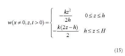
As best as I can tell, the derivation for this particular expression does not assume H to be constant in time, although it was derived for an already-existing ice sheet of (considerable) thickness H. Here, in order to be consistent with the notation used by Dansgaard and Johnsen, we are using H to represent the ice sheet height close to, but not directly at, the ice divide. Since the slope of the ice sheet is very shallow near the divide, H is a good approximation to the height of the ice sheet at the divide location. The value h is some fraction of H, usually 1/3 to 1/2 (Schwander et al., 2001, p. 4244). I assume that h is always the same fraction f of H(t) for all times t > 0, say h(t) = f‧H(t), although this assumption may "break down" for a very thin, nascent ice sheet. Applying the boundary condition that w(t) = -w_s(t) when z = H(t) allows us to obtain an expression for k(t), so that we can re-write Equation (for t > 0) as

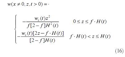
The time-rate of change of annual layer thicknesses is related to the partial derivative of w with respect to height z above bedrock,

Moreover in the absence of melting, the time rate of change of the height of the ice sheet must necessarily be the difference between the accumulation rate and the downward speed w_s(t) at the surface, and this must be true for all x and y:

Since the Mahaffy code specifies the accumulation rate for all x, y, and t, and since the Mahaffy code's output gives us H(x, y, t), Equation (8) may be used to obtain w_s(t) at the ice core's location. These values of w_s(t), together with the output values of H(t), may be inserted into Equations (16) and in order to calculate layer thicknesses as a function of time t and height z.

Some (very) preliminary work suggests that the amount of thinning in 4500 years near the center of an ice sheet is almost negligible, although I do not yet trust these preliminary calculations sufficiently to publish them. I invite careful scrutiny of my reasoning in this section of my paper.

In Hebert (2022), I expressed concern about using Mahaffy's model to estimate annual layer thicknesses, since Mahaffy's model assumes that the ice is deformed only by horizontal shear, ignoring both vertical shear and normal stresses/strains. However, normal stresses and strains cannot be ignored at an ice divide (Paterson, 1980, p. 43). Since horizontal velocity at the divide is always zero, there is no horizontal shear at the divide and, by symmetry, there is no vertical shear there, either. Rather, the ice layers are thinned via horizontal extension due to normal stresses (Cuffey and Paterson, 2010, p. 357).

However, this difficulty may be circumvented by using the model to determine layer thicknesses, not at the ice divide itself, but at some distance away from the divide. Moreover, Weertman (1961, p. 953) noted that these normal or longitudinal strains are only important for smaller ice sheets, about 30 kilometers in width. Since the Antarctic and Greenland ice sheets are much larger than this, it may still be possible to use the Mahaffey and Dansgaard-Johnsen models to obtain estimates of annual layer thicknesses near the center of a large ice sheet. Moreover, because the surface slope is very shallow for very large ice sheets, layer thicknesses calculated some small distance from the divide will probably also be good estimates for layer thicknesses at the divide location.

Although the Dansgaard-Johnsen model is an older one, it has been used even within the last twenty years or so (see Schwander et al., 2001) to provide preliminary estimates of annual layer thicknesses within the EPICA Dome C core.

The more sophisticated Blatter-Pattyn model (Blatter, 1995; Pattyn, 2003) could also be used for this purpose. It is my hope that perhaps other creation researchers will be able to build open these efforts, as estimates of these thicknesses could possibly enable us to strengthen the argument that the Greenland and Antarctic ice sheets are young.

Figure Captions

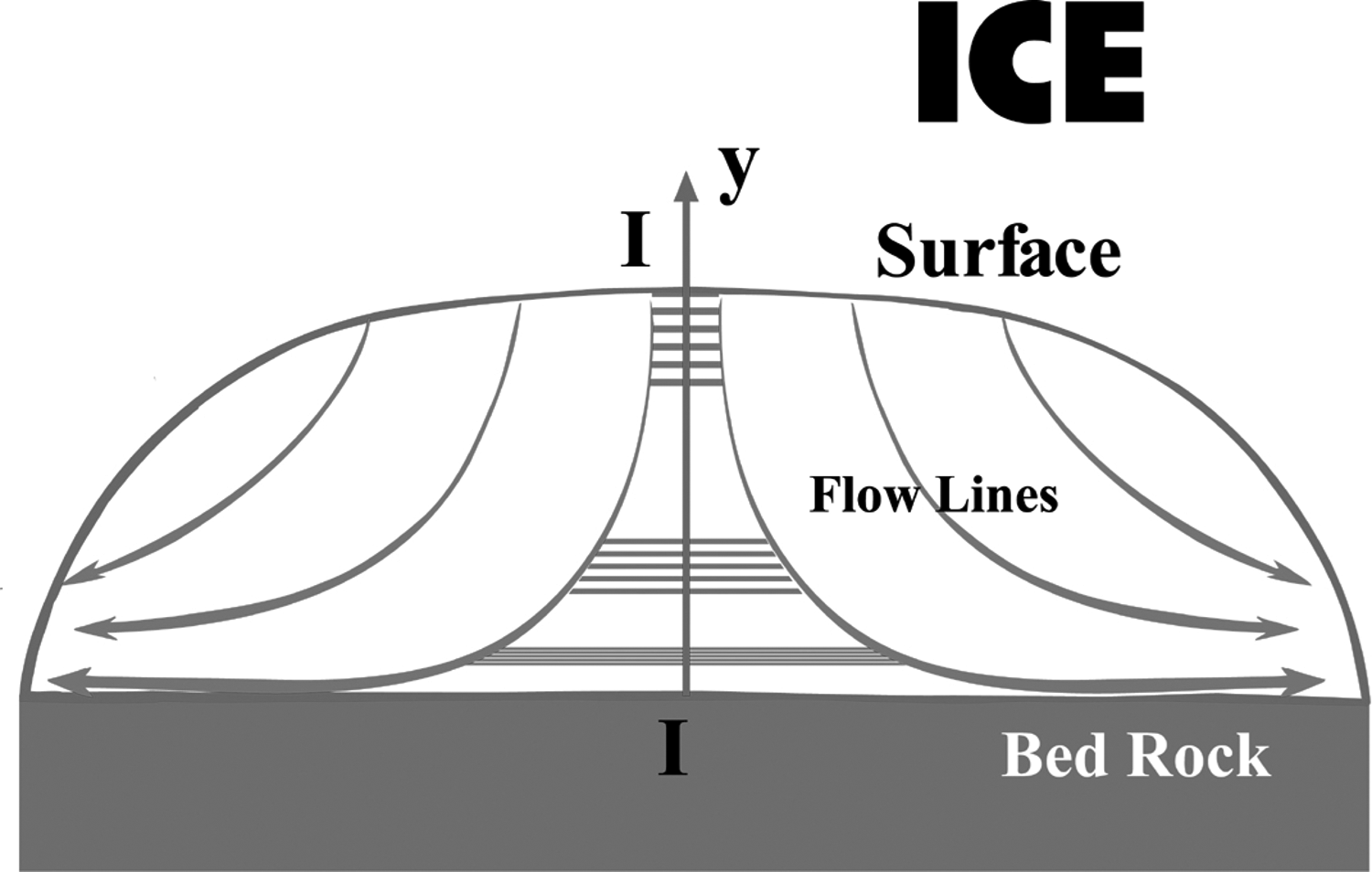
Figure 1. An idealized ice divide. Ice left of the divide flows to the left, and ice right of the divide flows to the right. Ice at the divide location must move straight down. Image courtesy of Michael J. Oard.

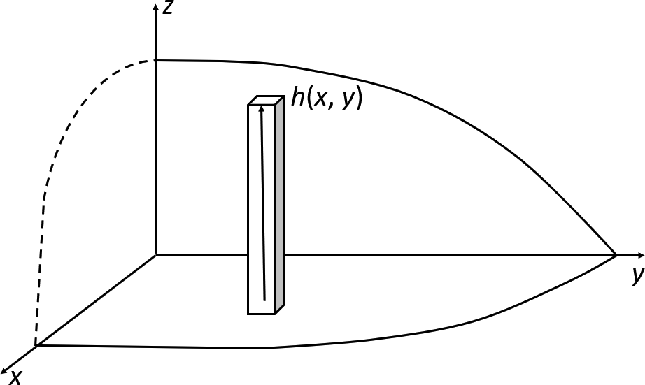
Figure 2. Coordinate system used in Mahaffy's ice-sheet model.

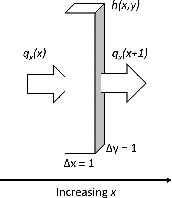
Figure 3. Horizontal fluxes (x-direction only) of ice flowing into and out of a column of ice.

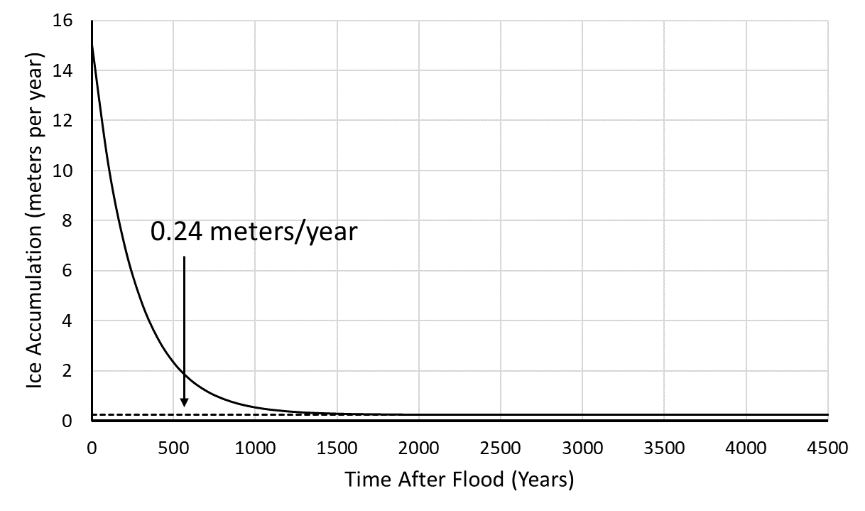
Figure 4. The accumulation rate (meters of ice per year) used in this exercise, calculated from Vardiman's model using values of Φ = 61.5, Ψ = 255 years, and λH/τ = 0.24 meters of ice per year. Note that the accumulation rate asymptotically approaches λH/τ = 0.24 meters/year as t goes to infinity.

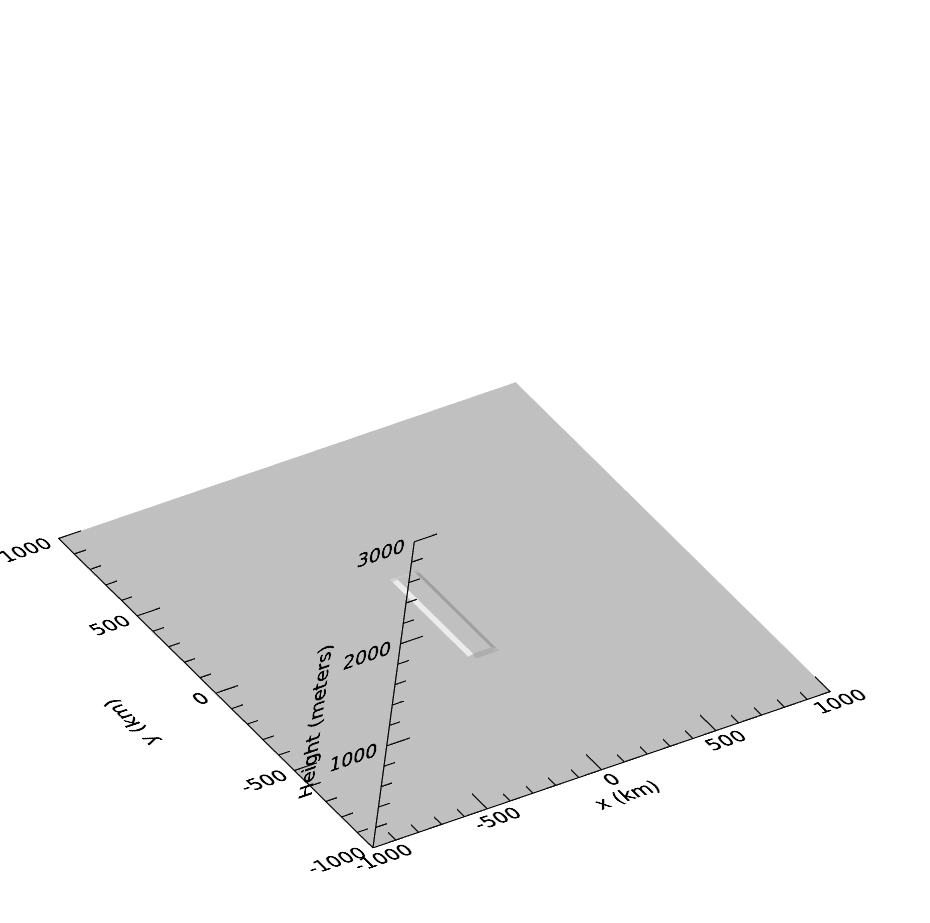
Figure 5. a) 15-meter-thick slab of ice deposited at t = 0 years after the Flood and the resulting ridge at b) t = 150 years after the Flood. The ridge height is greatly exaggerated compared to the ridge's horizontal dimensions.

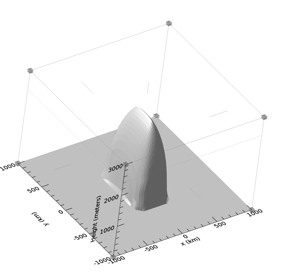
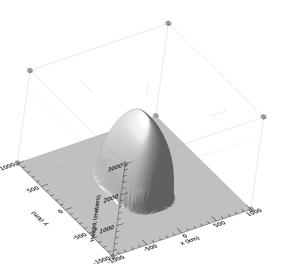
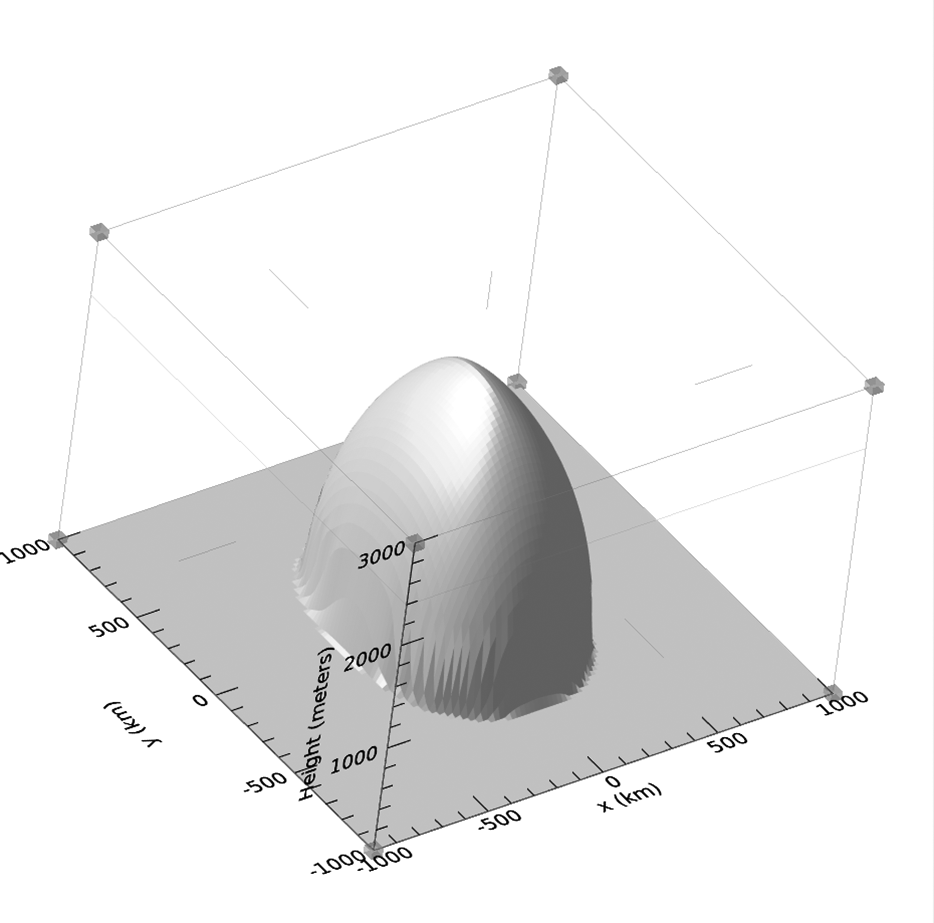
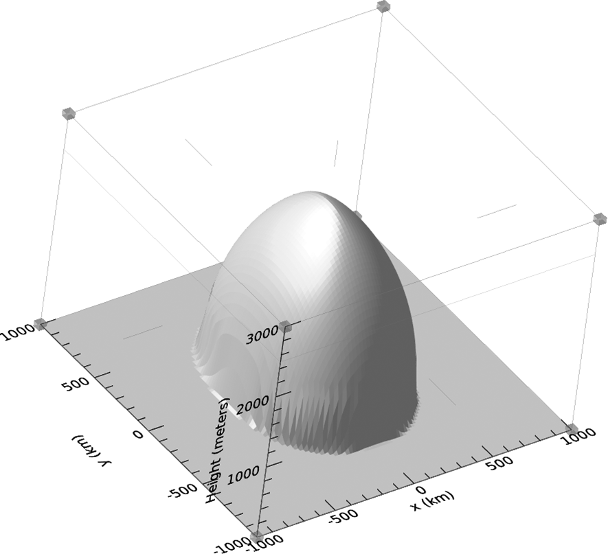
Figure 6. The ice ridge calculated from Mahaffy's model using Bueler's diffusive solution for a) 500 years, b) 1500 years, c) 3000 years, and d) 4500 years. The ridge height is greatly exaggerated compared to the ridge's horizontal dimensions.

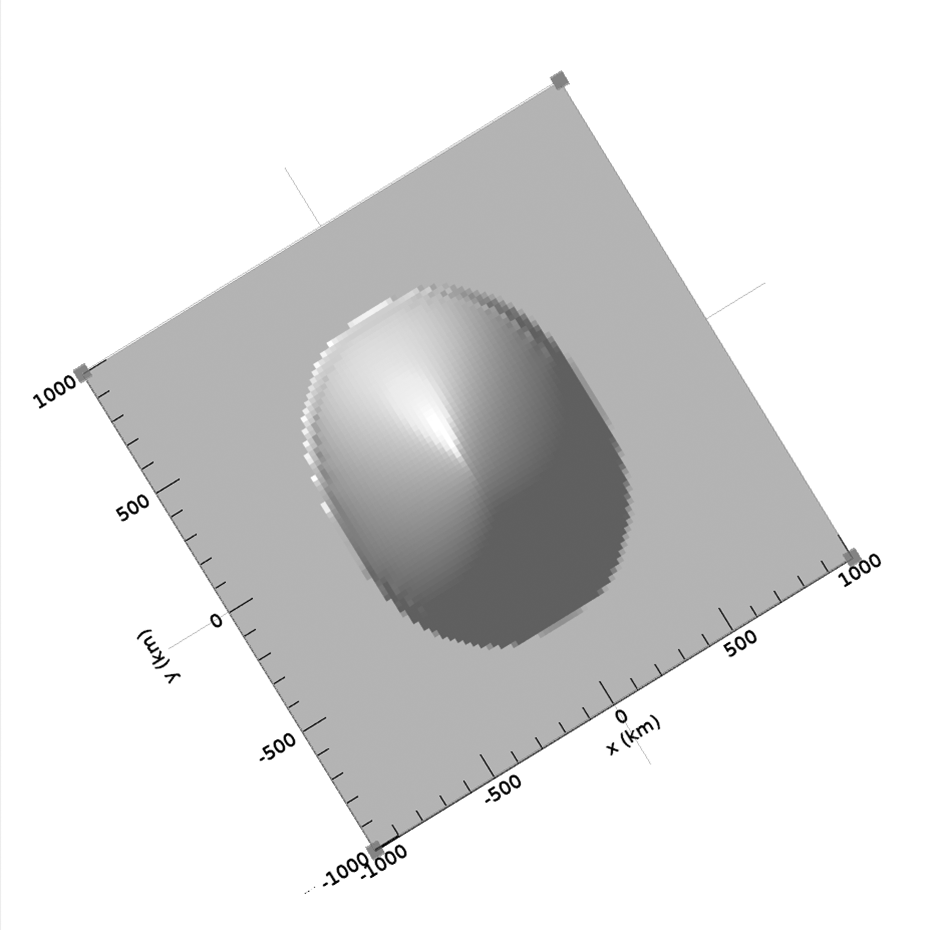
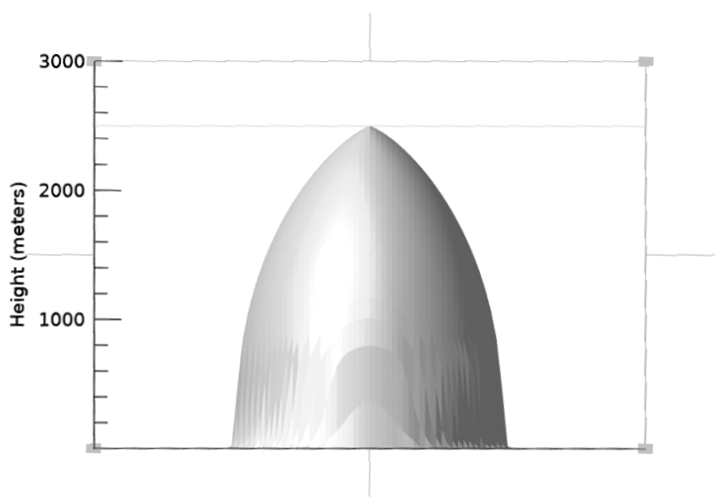
Figure 7. (a) Map view and (b) longitudinal view of ice ridge at t = 4500 years.

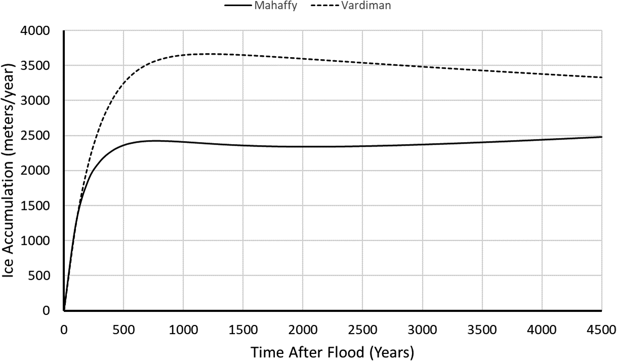
Figure 8. Height of the ice divide H as a function of time, calculated from both the Mahaffy and Vardiman models and using in both cases the values of Φ, Ψ, and λH/τ specified in the text and Figure 4.

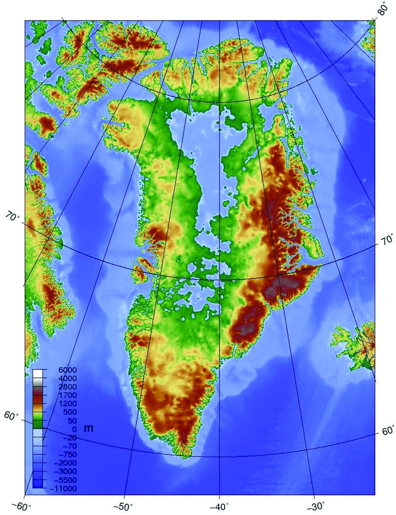
Figure 9. Bedrock topography for an ice-free Greenland. Image Credit: Skew-t, Wikimedia Commons. Creative Commons Attribution-Share Alike 3.0 Unported license. https://commons.wikimedia.org/wiki/File:Topographic_map_of_Greenland_bedrock.jpg.

References

Anonymous. Modelling the ice flow. Centre for Ice and Climate: Niels Bohr Institute. Posted on iceandclimate.nbi.ku.dk. (accessed December 29, 2021). [https://www.iceandclimate.nbi.ku.dk/research/strat_dating/forward_inv_modelling/.]

Bales, R.C., Q. Guo, D. Shen, J.R. McConnell, G. Du, J.F. Burkhart, V.B. Spikes, E. Hanna, and J. Cappelen. 2009. Annual accumulation for Greenland updated using ice core data developed during 2000-2006 and analysis of daily coastal meteorological data. Journal of Geophysical Research 114, D06116.

Blatter, H. 1995. Velocity and stress fields in grounded glaciers: A simple algorithm for including deviatoric stress gradients. Journal of Glaciology 41(138): 333 - 344.

Bueler, E. 2016. Numerical modelling of glaciers, ice sheets, and ice shelves. Notes for the International Summer School in Glaciology, McCarthy, Alaska. [https://glaciers.gi.alaska.edu/sites/default/files/notes-bueler-2016.pdf.]

Cuffey, K.M., and W.S.B. Paterson. 2010. The Physics of Glaciers (4th ed.). Butterworth-Heinemann (an imprint of Elsevier), Amsterdam, Netherlands.

Dansgaard, W., and S.J. Johnsen. 1969. A flow model and a time scale for the ice core from Camp Century, Greenland. Journal of Glaciology 8(53): 215-223.

Glen, J.W. 1955. The creep of polycrystalline ice. Proceedings of the Royal Society of London, Series A 228(1175): 519-538.

Hebert, J. 2021. Using Larry Vardiman's young-Earth ice-sheet model and a simple computer code to estimate annual layer thicknesses. Creation Research Society Quarterly 57(3): 175-185.

Hebert, J. 2022. Towards a more realistic young-Earth ice-sheet model: A shallow, isothermal ice dome with a frozen Base. Creation Research Society Quarterly 58(4): 262-272.

Mahaffy, M.W. 1976. A three-dimensional numerical model of ice sheets: Tests on the Barnes ice cap, Northwest Territories. Journal of Geophysical Research 81(6): 1059-1066.

Meese, D.A., A.J. Gow, R.B. Alley, G.A. Zielinski, P.M. Grootes, M. Ram, K.C. Taylor, P.A. Mayewski, and J.F. Bolzan. 1997. The Greenland Ice Sheet Project 2 depth-age scale: Methods and results. Journal of Geophysical Research 102(C12): 26411-26423.

Nye, J.F. 1952. The mechanics of glacier flow. Journal of Glaciology 2(11): 103-107.

Nye, J.F. 1957. The distribution of stress and velocity in glaciers and ice sheets. Proceedings of the Royal Society of London, Series A 239(1216): 477-489.

Oard, M.J. 2005. The Frozen Record: Examining the Ice Core History of the Greenland and Antarctic Ice Sheets. Institute for Creation Research, Santee, CA.

Oard, M.J. 2006. Frozen in Time: Woolly Mammoths, the Ice Age, and the Biblical Key to Their Secrets. (2nd printing). Master Books, Green Forest, AR.

Ohmura, A., and N. Reeh. 1991. New precipitation and accumulation maps for Greenland. Journal of Geophysical Research 37(25): 140-148. Cited in Oard (2005).

Paterson, W.S.B. 1980. Ice sheets and ice shelves. In Colbeck, Samuel C. (editor). 1980. Dynamics of Snow and Ice Masses. Academic Press, New York, NY.

Pattyn, F. 2003. A new three-dimensional higher-order thermomechanical ice sheet model: Basic sensitivity, ice stream development, and ice flow across subglacial lakes. Journal of Geophysical Research 108, No. B8. doi:10.1029/2002JB002329.

Schwander, J., J. Jouzel, C.U. Hammer, J.-R. Petit, R. Udisti, and E. Wolff. 2001. A tentative chronology for the EPICA Dome Concordia ice core. Geophysical Research Letters 28(22): 4243-4246.

Vardiman, L. 1993. Ice Cores and the Age of the Earth. Institute for Creation Research, San Diego, CA.

Vardiman, L. 1994. An analytic young-Earth flow model of ice-sheet formation during the "Ice Age." In Proceedings of the Third International Conference on Creationism. Walsh, Robert (editor). Creation Science Fellowship, Pittsburgh, PA, pp. 561-568.

Vardiman, L. 2001. Climates Before and After the Genesis Flood: Numerical Models and Their Implications. Institute for Creation Research, El Cajon, CA, pp. 41-68.